基于ggtreeExtra的环形进化树(circos plot)图片绘制

探索了ggtreeExtra这个R包,学习如何用其绘制环形进化树。

一、背景

是这样的。

最近想要绘制一些环形的图表(比方说下图,来自 DOI: 10.1126/sciadv.adq5038)。

image.png

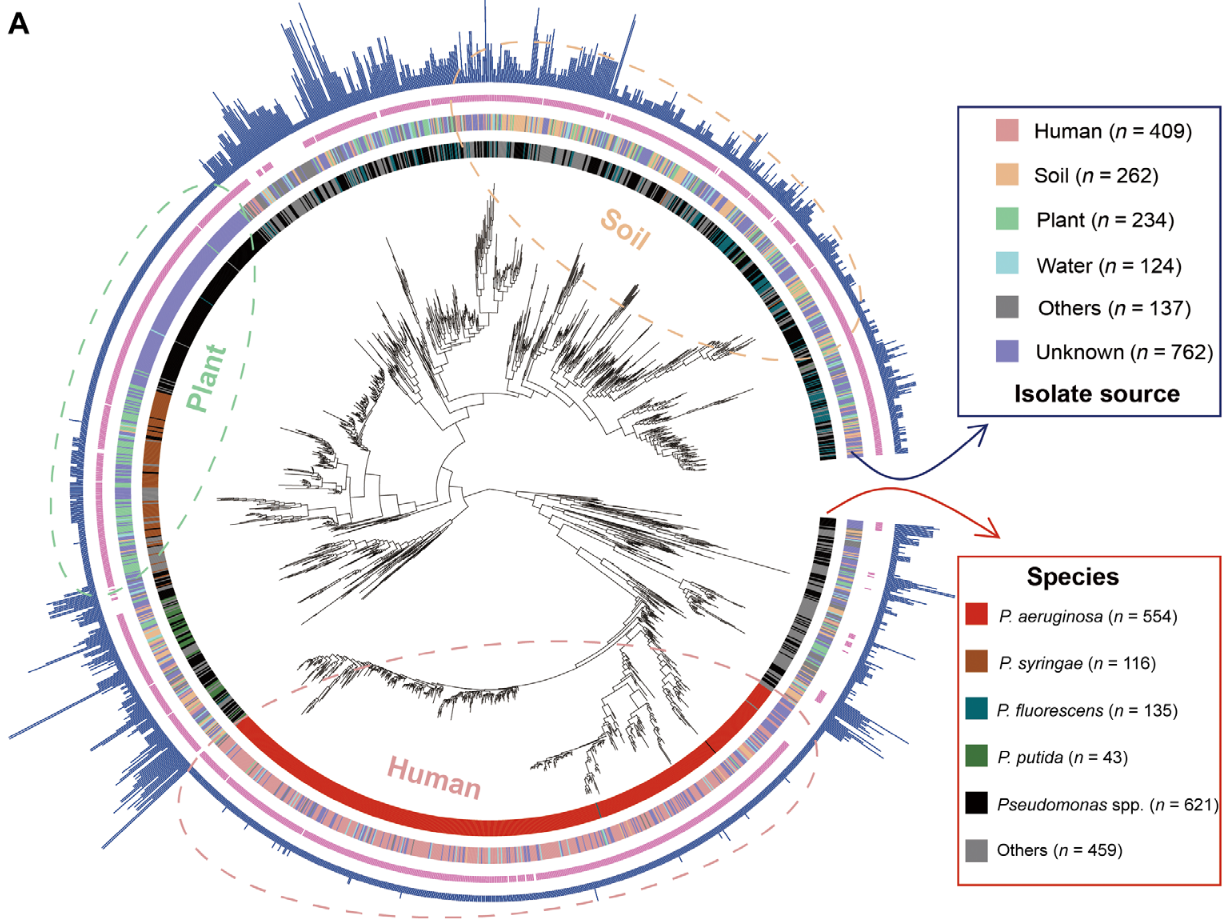
这种图片有个专门的名字,叫做circos plot,顾名思义就是把数据拼成一系列的圆环,看起来直观也好看。

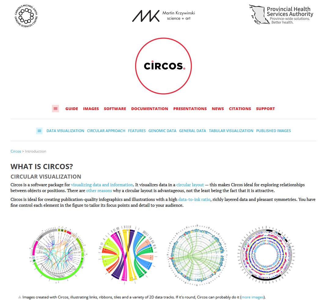
有一个用perl开发的专业软件叫做 circos.ca ,可以绘制这种图(如下图),笔者曾在大三的时候用过这个软件,它很专业,几乎所有的图表类型都可以画,而且样式多样,可以调得很美观。但说实话,这个软件太难用了,需要编写晦涩难懂的配置文件,并且渲染速度也很慢,因此这里不考虑。

image.png

另一个软件是ggtree,这是一个基于ggplot2的R包,可以绘制进化树,在往期博客中我们介绍过(见《使用ggtree绘制系统发育树》)。在这一次的学习和探索中,我发现ggtree还有一个Extra版本,可以绘制更为高端的图像,可以实现论文中的那种专业图片的效果。下面是探索记录

二、安装

主要需要用到的R包有下面这几个:

  • ape:进化树读取与处理
  • ggplot2:绘图的底层库
  • ggtree:绘制进化树
  • ggtreeExtra:绘制进化树外圈的circos plot

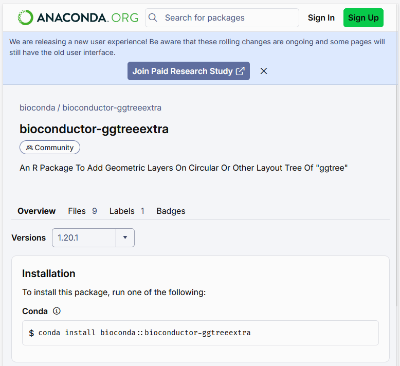
如果有conda,强烈建议使用conda安装上述R包(安装方法是去 anaconda.org 搜索包名,然后使用对应的指令进行安装,如下图)。

如果没有conda,那么需要借助 install.packages()BiocManager::install() 进行安装。其中,ape、ggplot2托管在CRAN上,使用 install.packages() 即可安装;ggtree和ggtreeExtra托管在bioconductor上,需要使用 BiocManager::install() 进行安装。

image.png

image.png

三、使用(代码示例)

下面是一个例子,在例子中展示了我们是如何一步一步绘制出带有进化树信息的circos plot的。

1
2
3
4
5
6
7
8
9
10
11
12
13
14
15
16
17
18
19
20
21
22
23
24
25
26
27
28
29
30
31
32
33
34
35
36
37
38
39
40
41
42
43
44
45
46
47
48
49
50
51
52
53
54
55
56
57
58
59
60
61
62
63
64
65
66
67
68
69
70
71
72
73
74
75
76
77
78
79
80
81
82
83
84
85
86
87
88
89
90
91
92
93
94
95
96
97
98
99
100
101
102
103
104
105
106
107
108
109
110
111
112
113
114
115
116
117
118
119
120
121
122
123
124
125
126
127
128
129

## 示例代码2(ggtreeExtra提供的示例树)
# 1. 加载核心包 (若无则需先安装: BiocManager::install("ggtreeExtra"))
library(ggtree)
library(ggtreeExtra)
library(ggplot2)
library(ggnewscale) # 用于重置颜色映射,避免冲突
library(ape) # 用于生成示例树数据
library(ggstar)
library(treeio)
# The path of tree file.
trfile <- system.file("extdata", "tree.nwk", package="ggtreeExtra")
# The path of file to plot tip point.
tippoint1 <- system.file("extdata", "tree_tippoint_bar.csv", package="ggtreeExtra")
# The path of first layer outside of tree.
ring1 <- system.file("extdata", "first_ring_discrete.csv", package="ggtreeExtra")
# The path of second layer outside of tree.
ring2 <- system.file("extdata", "second_ring_continuous.csv", package="ggtreeExtra")
# The tree file was imported using read.tree. If you have other tree format files, you can use corresponding functions from treeio package to read it.
tree <- read.tree(trfile)
# This dataset will to be plotted point and bar.
dat1 <- read.csv(tippoint1)
knitr::kable(head(dat1))
# This dataset will to be plotted heatmap
dat2 <- read.csv(ring1)
knitr::kable(head(dat2))
# This dataset will to be plotted heatmap
dat3 <- read.csv(ring2)
knitr::kable(head(dat3))
# The format of the datasets is the long shape for ggplot2. If you have short shape dataset,
# you can use `melt` of `reshape2` or `pivot_longer` of `tidyr` to convert it.
# We use ggtree to create fan layout tree.
p1 <- ggtree(tree, layout="fan", open.angle=10, size=0.5)
#> Scale for y is already present.
#> Adding another scale for y, which will replace the existing scale.
p1
p2 <- p1 +
geom_fruit(
data=dat1,
geom=geom_star,
mapping=aes(y=ID, fill=Location, size=Length, starshape=Group),
position="identity",
starstroke=0.2
) +
scale_size_continuous(
range=c(1, 3), # the range of size.
guide=guide_legend(
keywidth=0.5,
keyheight=0.5,
override.aes=list(starshape=15),
order=2
)
) +
scale_fill_manual(
values=c("#F8766D", "#C49A00", "#53B400", "#00C094", "#00B6EB", "#A58AFF", "#FB61D7"),
guide="none"
) +
scale_starshape_manual(
values=c(1, 15),
guide=guide_legend(
keywidth=0.5,
keyheight=0.5,
order=1
)
)
p2
p3 <- p2 +
new_scale_fill() +
geom_fruit(
data=dat2,
geom=geom_tile,
mapping=aes(y=ID, x=Pos, fill=Type),
offset=0.08, # The distance between external layers, default is 0.03 times of x range of tree.
pwidth=0.25 # width of the external layer, default is 0.2 times of x range of tree.
) +
scale_fill_manual(
values=c("#339933", "#dfac03"),
guide=guide_legend(keywidth=0.5, keyheight=0.5, order=3)
)
p3
# You can also add heatmap layer for continuous values.
p4 <- p3 +
new_scale_fill() +
geom_fruit(
data=dat3,
geom=geom_tile,
mapping=aes(y=ID, x=Type2, alpha=Alpha, fill=Type2),
pwidth=0.15,
axis.params=list(
axis="x", # add axis text of the layer.
text.angle=-45, # the text angle of x-axis.
hjust=0 # adjust the horizontal position of text of axis.
)
) +
scale_fill_manual(
values=c("#b22222", "#005500", "#0000be", "#9f1f9f"),
guide=guide_legend(keywidth=0.5, keyheight=0.5, order=4)
) +
scale_alpha_continuous(
range=c(0, 0.4), # the range of alpha
guide=guide_legend(keywidth=0.5, keyheight=0.5, order=5)
)
p4
# Then add a bar layer outside of the tree.
p5 <- p4 +
new_scale_fill() +
geom_fruit(
data=dat1,
geom=geom_col,
mapping=aes(y=ID, x=Abundance, fill=Location), #The 'Abundance' of 'dat1' will be mapped to x
pwidth=0.4,
axis.params=list(
axis="x", # add axis text of the layer.
text.angle=-45, # the text size of axis.
hjust=0 # adjust the horizontal position of text of axis.
),
grid.params=list() # add the grid line of the external bar plot.
) +
scale_fill_manual(
values=c("#F8766D", "#C49A00", "#53B400", "#00C094", "#00B6EB", "#A58AFF", "#FB61D7"),
guide=guide_legend(keywidth=0.5, keyheight=0.5, order=6)
) +
theme(#legend.position=c(0.96, 0.5), # the position of legend.
legend.background=element_rect(fill=NA), # the background of legend.
legend.title=element_text(size=7), # the title size of legend.
legend.text=element_text(size=6), # the text size of legend.
legend.spacing.y = unit(0.02, "cm") # the distance of legends (y orientation).
)
p5

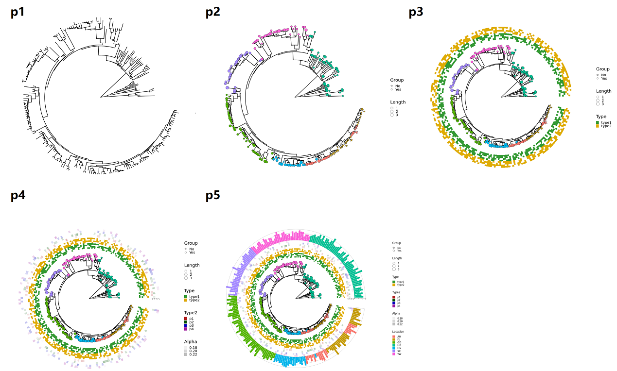
我们可以注意到,代码中分了多个步骤,依次绘制了p1到p5。ggplot2的绘图语法是一种声明式的语法,允许用户使用“+”(加号)在一个绘图对象上增加新的东西,因此我们可以在每一个步骤中增加圆环的数量,层层递进。

在上述代码中, geom_fruit() 这个函数是其中最为关键的函数,其名称很形象(绘制一颗环形进化树外圈数据的过程,就像在一棵树上挂果实一样),通过 mapping 参数可以指定如何对齐进化树的树枝以及对应的数据点。举一个例子, mapping=aes(y=ID, x=Type2) ,这里就是说使用数据里面的ID这一列去对齐进化树的树枝,而 x=Type2 是需要可视化的数据。

下面是p1到p5的全部内容:

image.png

四、讨论

相比于基于perl编程语言的 circos.ca ,ggtreeExtra的性能要好许多,并且借助ggplot2强大的图形库与调色板功能,可以绘制出非常好看的图像,因此这个包是绘制环形进化树统计图的非常好的选择。

实际使用中,我们可以把数据存储为nwk格式(进化树)和csv(需要可视化的外层数据),只要进化树的叶子节点的ID能够与数据中的记录ID(用mapping参数指定的那个)一一对应起来即可。这里面需要留意的问题是,在一些数据源中,物种名称的属名与种加词(Genus and species name)是使用空格字符相连接的(比方说, “Homo sapiens” ) ,另一些数据源中则以下划线相连(如 “Homo_sapiens” ),这种不同之处会导致mapping的时候对应不上,需要预先转换——所以我们在绘图前需要检查数据。

总的来说,这是一个很好的工具,强烈推荐有需要的朋友试用。