如题。
前段时间休假在家,学习了不少心理学方面的知识,某日突然有一个疑惑:我算是一个情绪稳定的人吗?或者说,我想知道自己的情绪稳定性,在这些年来是变得更稳定了,还是更不稳定了。当我把这一疑问提交给chatGPT以后,它告诉我,可以分析一下这几年来的日记中的情感倾向变化,从而更好的了解自己。于是对文本情感倾向性分析进行了一些探索。
一、基于textblob的文本倾向性分析 textblob 是一个用于文本数据(textual data)处理的python库,其提供了一系列自然语言处理的函数,包括文本情感分析。要使用这个库也很简单,只需要pip install textblob即可完成安装,随后使用下面的代码就可以完成文本的情感倾向性分析。
1
2
3
4
5
6
from textblob import TextBlobtestimonial = TextBlob("Textblob is amazingly simple to use. What great fun!" ) print (testimonial.sentiment)print (testimonial.sentiment.polarity)
上述函数接口传入一段文本,返回一个(polarity,subjectivity)元组,其中polarity代表极性得分,值域为[-1.0,1.0] ,代表情感倾向性;subjectivity代表主观性得分,值域为[0.0,1.0],其中0代表非常客观,1代表非常主观。
不过这个库有缺点,只能处理英文文本,因此这里不考虑使用。
二、基于snowNLP的中文文本倾向性分析
参考: 情感分析——深入snownlp原理和实践
受textblob启发,有国人针对中文场景开发了一个文本处理的python库,叫做snowNLP 。安装方法同样很简单,pip install snownlp 即可。下面是一个使用方法示例:
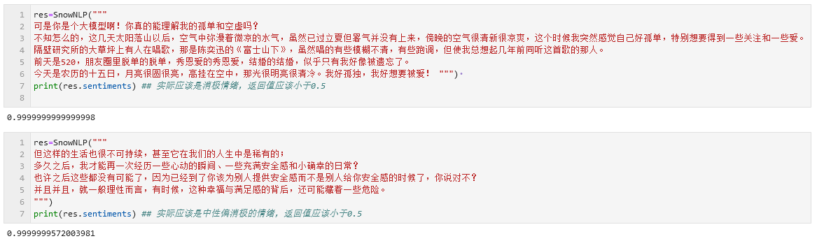
1
2
3
4
5
6
7
from snownlp import SnowNLPres=SnowNLP("北京连着下了三天的雪,今天晚上终于停了" ) print (res.sentiments)res=SnowNLP("这个东西真心很赞" ) print (res.sentiments)
上述函数接口传入一段文本,返回一个浮点数,代表文本属于积极情绪的概率值。
然而snowNLP也存在缺点,因为作者是在电商评论数据集上训练的模型,因此在日记文本上的分类非常不准确,几乎会把任何传入的文本分类为积极情绪(如下图)。此外,传入文本的长度似乎也会影响snowNLP的分类情况,文本越长snowNLP给出的积极性评分也越高(即使是同一段文本内容,重复次数越多得分也越高)。因此这里同样不考虑使用。
三、百度智能云的解决方案 幸运的是,我们还有百度提供的API接口。参考:
百度智能云 - 情感倾向分析
这一API能够对只包含单一主体主观信息的文本,进行自动情感倾向性判断(积极、消极、中性),并给出相应的置信度。为口碑分析、话题监控、舆情分析等应用提供基础技术支持。其通过HTTPS的POST请求进行调用,请求URL为 https://aip.baidubce.com/rpc/2.0/nlp/v1/sentiment_classify , payload格式如下:
上述API的返回值是一个json文档,其结构如下:
1 2 3 4 5 6 7 8 9 10 11 { "text" : "我爱祖国" , "items" : [ { "sentiment" : 2 , "confidence" : 0.90 , "positive_prob" : 0.94 , "negative_prob" : 0.06 } ] }
因此,我们可以很方便的构建分析函数,如下:
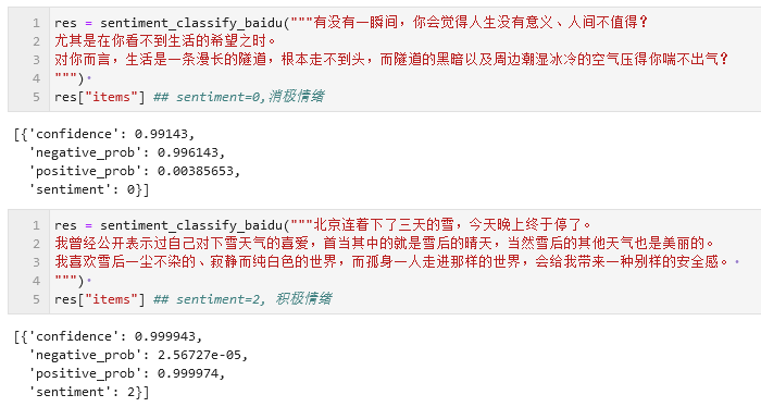
1 2 3 4 5 6 7 8 9 10 11 12 13 14 15 16 17 18 19 20 21 22 23 24 25 import requestsimport jsonAPI_Key = "xxxxxx" Secret_Key = "xxxxxx" headers = { 'Content-Type' : 'application/json' , 'Accept' : 'application/json' , 'User-Agent' :'Mozilla/5.0 (Windows NT 10.0; Win64; x64; rv:109.0) Gecko/20100101 Firefox/115.0' } def get_access_token (): url = "https://aip.baidubce.com/oauth/2.0/token?grant_type=client_credentials&client_id={}&client_secret={}" .format (API_Key,Secret_Key) payload = json.dumps("" ) response = requests.request("POST" , url, headers=headers, data=payload) return response.json().get("access_token" ) def sentiment_classify_baidu (text ): url = "https://aip.baidubce.com/rpc/2.0/nlp/v1/sentiment_classify?charset=UTF-8&access_token=" + get_access_token() dt = { "text" : text } payload = json.dumps(dt) response = requests.request("POST" , url, headers=headers, data=payload) res = response.json() return res
相比于snowNLP,百度的API很显然在训练时使用了更加广泛的语料库,因此分析结果也基本上是准确的。
四、分析结果与讨论 (一)情感倾向性分析 基于前面的探索,我们可以基于百度的API进行情感倾向性分析。
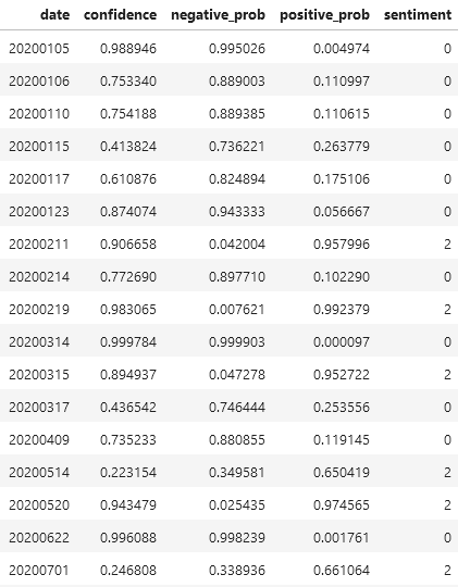
我们可以批量读取日记的文本内容,使用上述代码计算情感倾向性,并按日期汇总为一个dataframe(如下图),以便后续分析。此处可以将dataframe导出为csv格式备用。(代码略)
(二)如何定义“情绪稳定性” 每一篇日记都代表一个孤立的时间点。单独一篇日记的情感倾向性并不能说明什么,只有分析一段时间内的情感倾向性变化才有意义。
因此,对“情绪稳定性”的度量可以转变为下述问题:对于一串代表情感倾向性的序列向量,如何衡量其变化过程的平稳性?
(一个直观点的描述是这样:假设某段时间内的情感倾向性变化过程是[0,0,0,2,2,2],代表一段稳定的 消极情绪过后是一段很稳定的积极情绪,另一段时间内的情感倾向性变化过程是 [0,2,0,2,0,2],代表两种情绪交替出现,情绪稳定性很差。那么,如何在统计指标上体现出这种差异。)
我们可以定义一个 情绪转换率(emotion conversion rate) 。其定义为情绪转换次数与序列长度的比值。例如序列[0,0,0,2,2,2]中,情绪转换1次,情绪转换率为1/6;序列 [0,2,0,2,0,2]中,情绪转换5次,情绪转换率为5/6。这个指标提供了一个标准化的度量,使得不同长度的序列之间可以进行比较。
需要注意的是,实际计算时,从消极情绪(0)转移到积极情绪(2)会被算作两次而不是一次,因为这样的情绪转换跨过了中性情绪(1)。
在计算情绪转换率的过程中,可以使用numpy.diff()函数提高效率。
(三)滑窗分析与最终结果 下面是滑窗分析的代码。需要事先准备好日记情感倾向性分析结果的dataframe(见上文),下面的代码会基于用户给定的时间段和窗口长度,对一段时间内的 情感倾向变化情况 以及 情绪转换率 进行计算。
1 2 3 4 5 6 7 8 9 10 11 12 13 14 15 16 17 18 19 20 21 22 23 24 25 26 27 28 29 30 31 32 33 34 35 36 37 38 39 40 41 42 43 44 45 46 47 48 49 50 51 52 53 54 55 56 57 58 59 60 61 62 63 64 65 66 67 68 69 70 71 72 73 74 75 76 77 78 79 80 81 82 83 84 85 86 87 88 89 90 91 92 93 94 95 96 97 98 99 100 101 102 103 104 105 106 107 108 109 110 import os,sys,timefrom matplotlib import pyplot as pltfrom matplotlib.gridspec import GridSpecimport numpy as npimport pandas as pdstart_date = "20200101" end_date = "20220630" start_stamp = int (time.mktime(time.strptime(start_date,"%Y%m%d" ))) end_stamp = int (time.mktime(time.strptime( end_date,"%Y%m%d" ))) one_day_stamp = abs ( \ int (time.mktime(time.strptime("20200101" ,"%Y%m%d" ))) - \ int (time.mktime(time.strptime("20200102" ,"%Y%m%d" ))) ) time_stamps_list = [] for d in sentiment_analysis_baidu_df["date" ]: time_stamps_list.append(int (time.mktime(time.strptime(str (d),"%Y%m%d" )))) date_list = list (sentiment_analysis_baidu_df["date" ]) def get_n_day_average (day_stamp,n=30 ): stamp0 = int (day_stamp-one_day_stamp*n/2 ) stamp1 = int (day_stamp+one_day_stamp*n/2 ) negative_prob_list = [] positive_prob_list = [] sentiment_list = [] for stamp in range (stamp0,stamp1,one_day_stamp): date_num = int (time.strftime("%Y%m%d" ,time.localtime(stamp))) if (date_num in date_list): data_row = sentiment_analysis_baidu_df[sentiment_analysis_baidu_df["date" ]==date_num] neg_prob = float (data_row["negative_prob" ]) pos_prob = float (data_row["positive_prob" ]) sentiment = int (data_row["sentiment" ]) negative_prob_list.append(neg_prob) positive_prob_list.append(pos_prob) sentiment_list.append(sentiment) neg_avg = np.mean(negative_prob_list) pos_avg = np.mean(positive_prob_list) sentiment_avg = np.mean(sentiment_list) emo_conv_rate = np.sum (np.abs (np.diff(sentiment_list)))/n return (neg_avg,pos_avg,sentiment_avg,emo_conv_rate) def analysis (window_size=30 ,start_date="20200101" ,end_date="20220630" ): start_stamp = int (time.mktime(time.strptime(start_date,"%Y%m%d" ))) end_stamp = int (time.mktime(time.strptime( end_date,"%Y%m%d" ))) one_day_stamp = abs ( \ int (time.mktime(time.strptime("20200101" ,"%Y%m%d" ))) - \ int (time.mktime(time.strptime("20200102" ,"%Y%m%d" ))) ) x_date_list = [] neg_avg_list = [] pos_avg_list = [] sentiment_avg_list = [] emo_conv_rate_list = [] for stamp in range (start_stamp,end_stamp,one_day_stamp): date_num = int (time.strftime("%Y%m%d" ,time.localtime(stamp))) x_date_list.append(date_num) neg_avg,pos_avg,sentiment_avg,emo_conv_rate = get_n_day_average(stamp,window_size) neg_avg_list.append(neg_avg) pos_avg_list.append(pos_avg) sentiment_avg_list.append(sentiment_avg) emo_conv_rate_list.append(emo_conv_rate) res_df = pd.DataFrame({"date" :x_date_list, "negative_prob" :neg_avg_list, "positive_prob" :pos_avg_list, "sentiment" :sentiment_avg_list, "emotion_conv_rate" :emo_conv_rate_list}) return res_df def plot_df (res_df,title ): x = np.arange(res_df.shape[0 ]) fig = plt.figure(figsize=[19.2 , 10.8 ], constrained_layout=True , tight_layout=True ) gs = GridSpec(4 ,1 ,figure=fig,wspace=0 ,hspace=0 ) ax1 = fig.add_subplot(gs[0 :1 ,0 :1 ]) ax1.plot(x,res_df["negative_prob" ],color="#eff08a" ) ax1.set_ylabel("negative_prob" ) plt.title(title) ax2 = fig.add_subplot(gs[1 :2 ,0 :1 ]) ax2.plot(x,res_df["positive_prob" ],color="#ff8a8a" ) ax2.set_ylabel("positive_prob" ) ax3 = fig.add_subplot(gs[2 :3 ,0 :1 ]) ax3.plot(x,res_df["sentiment" ] ,color="#8ab9ff" ) ax3.set_ylabel("sentiment" ) ax4 = fig.add_subplot(gs[3 :4 ,0 :1 ]) ax4.plot(x,res_df["emotion_conv_rate" ],color="#b9ff8a" ) ax4.set_ylabel("emotion_conv_rate" ) ax4.set_xlabel("date" ) x_ = [] date_ = [] for i in range (0 ,res_df.shape[0 ],30 ): x_.append(x[i]) date_.append(int (res_df.iloc[i,:]["date" ])) plt.xticks(x_,date_,rotation=60 ) plt.savefig(f"report_{title} .png" ) plt.show()
使用方法如下:
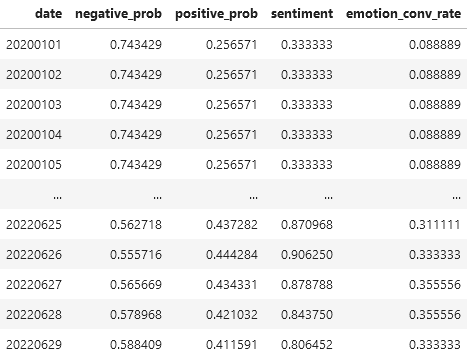
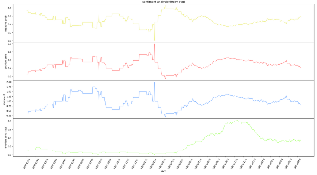
1 2 3 4 5 6 7 8 sentiment_analysis_baidu_df = pd.read_csv("sentiment_analysis_baidu_df.txt" ,sep="\t" ) flip_window_df = analysis(window_size=90 ,start_date="20200101" ,end_date="20220630" ) display(flip_window_df) plot_df(flip_window_df,title="sentiment analysis(90day avg)" )
绘制出来的曲线长下图这个样子(图片仅为示例)。
根据曲线可以判断出来,我确实是一个情绪不太稳定的人,特别是在大四上半学期(2021年10月左右),情绪不稳定性在持续走高😭(看图中最下面的绿线,那段时间存在非常明显的上扬趋势)。
至于现在呢?——
研究生期间的曲线就不放了。说出来丢人,单看情绪转换率这个指标的话,现阶段我的情绪稳定性确实比大学刚毕业那会儿要好不少,但在某些时间段也有一些波动和起伏。
而且想了下,这样的分析可能也存在问题。“情绪转换率”这个指标可能并不完美,文本情感倾向性分析也太局限了。特别是,把自己的情绪波动量化为冷冰冰的数字,虽然听起来很有创意、很极客,但是否有些不近人情呢?
或许在情商的锻炼上,我还有很长的路要走吧。
以上。